Back to top
Objective
The objective of this post is to systematically derive the corresponding parametric equations and implement them in Python for visualization using Manim. The aim is not only to develop a clear analytical understanding of these curves, but also to bring them to life through computational animation.
Back to top
Definition
Cycloidal curves are the loci of a fixed point on the circumference of a circle as it rolls without slipping along a given path. Depending on whether the circle rolls along a straight line, on the outside of another circle, or on the inside of another circle, the resulting curve is classified as a cycloid, an epicycloid, or a hypocycloid.
 Cardioid
 ($r = R$), a special case of the epicycloid.
Back to top
Cycloid
Parametric equations:
$x(\theta) = r(\theta - \sin \theta)$
$y(\theta) = r(1 - \cos \theta)$
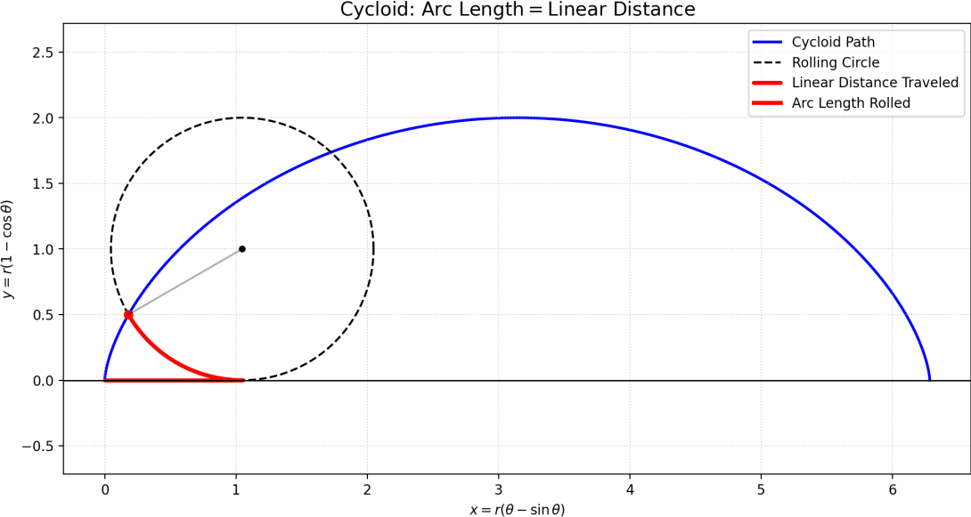
A cycloid is the curve traced by a point on the circumference of a circle as it rolls along a straight line (the directrix) without slipping.
In engineering, the cycloid is notable for its brachistochrone property—representing the path of fastest descent under gravity—and its tautochrone property, where the time taken by a particle to reach the lowest point is independent of its starting position.
Derivation of Parametric Equations of Cycloid
$s = r\theta$
$a = r \cos \theta$
$b = r \sin \theta$
$x = s - b = r\theta - r \sin \theta$
$x = r(\theta - \sin \theta)$
$y = r - a = r - r \cos \theta)$
$y = r(1 - \cos \theta)$
Area and Length of Arc of a Cycloid
The length of arc and area of a cycloid, by integration, is posted at node 2353.
Manim Code for Cycloid
The scripts provided below were developed with AI assistance and were carefully reviewed to ensure alignment with the mathematical principles discussed.
Video Output of Manim Code for Cycloid
Note: The visual branding shown in the videos (e.g. MATHalino logo) is not included in the shared Manim code to keep the scripts clean and reusable.
Back to top
Epicycloid
Parametric equations:
$x(\theta) = (R + r) \cos \theta - r \cos \left( \dfrac{R + r}{r} \theta \right)$
$y(\theta) = (R + r) \sin \theta - r \sin \left( \dfrac{R + r}{r} \theta \right)$
An epicycloid is a plane curve generated by a point on the circumference of a circle (the generating circle) that rolls along the exterior of a fixed circle (the base circle). The shape of the resulting path is determined by the ratio of the radii of the two circles. A common application of the epicycloid is in the profile of planetary gears and certain types of rotary pumps.
Derivation of Parametric Equations of Epicycloid
$s_2 = s_1$
$r \alpha = R \theta$
$\alpha = \dfrac{R \theta}{r}$
$x_1 = (R + r) \cos \theta$
$\begin{align}x_2 & = r \cos (\alpha + \theta) = r \cos \left(\dfrac{R \theta}{r} + \theta \right) \\
& = r \cos \left(\dfrac{R + r}{r} \theta \right)\end{align}$
$x = x_1 - x_2$
$x = (R + r) \cos \theta - r \cos \left(\dfrac{R + r}{r} \theta \right)$
$y_1 = (R + r) \sin \theta$
$\begin{align}y_2 & = r \sin (\alpha + \theta) = r \sin \left(\dfrac{R \theta}{r} + \theta \right) \\
& = r \sin \left(\dfrac{R + r}{r} \theta \right)\end{align}$
$y = y_1 - y_2$
$y = (R + r) \sin \theta - r \sin \left(\dfrac{R + r}{r} \theta \right)$
Distance from the Origin to a Point on the Epicycloid
${R_C}^2 = x^2 + y^2$
From the parametric equations:
$x = (R + r) \cos \theta - r \cos \left(\dfrac{R + r}{r} \theta \right)$
$y = (R + r) \sin \theta - r \sin \left(\dfrac{R + r}{r} \theta \right)$
Let
$a = R + r$ and $b = \dfrac{R + r}{r}$
The parametric equations will become
$x = a \cos \theta - r \cos b\theta$
$y = a \sin \theta - r \sin b\theta$
$x^2 = (a \cos \theta - r \cos b\theta)^2$
$x^2 = a^2 \cos^2 \theta - 2ar \cos \theta \cos b\theta + r^2 \cos^2 b\theta$
$y^2 = (a \sin \theta - r \sin b\theta)^2$
$y^2 = a^2 \sin^2 \theta - 2ar \sin \theta \sin b\theta + r^2 \sin^2 b\theta$
${R_C}^2 = (a^2 \cos^2 \theta - 2ar \cos \theta \cos b\theta + r^2 \cos^2 b\theta) + (a^2 \sin^2 \theta - 2ar \sin \theta \sin b\theta + r^2 \sin^2 b\theta)$
${R_C}^2 = a^2 (\sin^2 \theta + \cos^2 \theta) + r^2 (\sin^2 b\theta + \cos^2 b\theta) - 2ar (\cos \theta b\cos \theta + \sin \theta \sin b\theta)$
${R_C}^2 = a^2 (1) + r^2 (1) - 2ar (\cos b\theta \cos \theta + \sin b\theta \sin \theta)$
Use the difference of two angles:
$\cos A \cos B + \sin A \sin B = \cos (A - B)$
For $A = b\theta$ and $B = \theta$:
$\cos b\theta \cos \theta + \sin b\theta \sin \theta = \cos (b - 1)\theta$
Let $k = b - 1$
$k = \dfrac{R + r}{r} - 1 = \dfrac{R + r - r}{r} = \dfrac{R}{r}$
$\cos b\theta \cos \theta + \sin b\theta \sin \theta = \cos k\theta$
Hence,
${R_C}^2 = a^2 + r^2 - 2ar \cos k\theta$
$R_C = \sqrt{a^2 + r^2 - 2ar \cos k\theta}$
Limits of Integration (Epicycloid and Hypocycloid)
The calculations below have been verified by MATHalino for $r \le R$. No verification has yet been carried out by MATHalino for the case $r \gt R$.
Central Angle for One Rotation
When the circle of radius $r$ completes one full rotation while rolling on the circle of radius $R$, it travels a distance of $2\pi r$. This arc length on the fixed circle subtends an angle $\alpha$ at its center, so
$$R\alpha = 2\pi r$$
from which
$$\alpha = \dfrac{2\pi r}{R} = \dfrac{2\pi}{R/r} = \dfrac{2\pi}{k}$$
Therefore, for one complete rotation of the rolling circle, the limit of integration is from $0$ to $2\pi /k$.
Number of Cusps (Epicycloid and Hypocycloid)
The number of cusps depends on the ratio $R/r$. Writing $R = nr$, the number of cusps is equal to $n$ when $n$ is an integer.
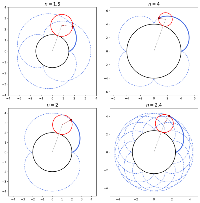 Epicycloids with varying values of $n$
For non-integer $n$, write the ratio in lowest terms as $p/q$. The number of cusps is then $p$, while the number of revolutions required for the graph to close is $q$. If $R/r$ is irrational, the number of cusps is infinite because the graph never closes.
Area of Epicycloid
The area of an epicycloid is the region between the epicycloidal curve and the fixed circle. In other words, it is the area inside the epicycloid but outside the fixed circle.
For cases with no overlapping cusps, the total area of the epicycloid is equal to $n$ times the area of one cusp.
Differential Area of Epicycloid
$dA = \frac{1}{2}({R_C}^2 - R^2) \, d\theta$
$dA = \frac{1}{2} \left[ (a^2 + r^2 - 2ar \cos k\theta) - R^2 \right] \, d\theta$
$dA = \frac{1}{2} \left[ (a^2 + r^2 - R^2) - 2ar \cos k\theta \right] \, d\theta$
$dA = \left( \dfrac{a^2 + r^2 - R^2}{2} - ar \cos k\theta \right) \, d\theta$
Area of One Cusp of Epicycloid
The area between the fixed circle and the epicycloid arc is the shaded region in the figure above. This region is outside the fixed circle but inside the epicycloid.
$A = \displaystyle \dfrac{a^2 + r^2 - R^2}{2} \int_0^{2\pi / k} d\theta - ar \int_0^{2\pi / k} \cos k\theta \, d\theta$
$A = \displaystyle \dfrac{a^2 + r^2 - R^2}{2} \left[ \theta \right]_0^{2\pi / k} - \dfrac{ar}{k}\left[ \sin k\theta \right]_0^{2\pi / k}$
$A = \displaystyle \dfrac{a^2 + r^2 - R^2}{2} \left[ \dfrac{2\pi}{k} - 0 \right] - \dfrac{ar}{k}\left[ \sin \left( k \cdot \dfrac{2\pi}{k} \right) - \sin 0 \right]$
$A = \displaystyle \dfrac{a^2 + r^2 - R^2}{2} \left[ \dfrac{2\pi}{R/r}\right] - \dfrac{ar}{R/r}\left[ \sin (2\pi) \right]$
$A = (a^2 + r^2 - R^2) \cdot \dfrac{\pi r}{R}$
$A = \left[ (R + r)^2 + r^2 - R^2 \right] \cdot \dfrac{\pi r}{R}$
$A = \left[ (R^2 + 2Rr + r^2) + r^2 - R^2 \right] \cdot \dfrac{\pi r}{R}$
$A = (2Rr + 2r^2) \cdot \dfrac{\pi r}{R}$
$A = 2r(R + r) \cdot \dfrac{\pi r}{R}$
$A = 2 \left( \dfrac{R + r}{R} \right) \pi r^2$
For $R = 3$ and $r = 1$:
$A = 2 \left( \dfrac{3 + 1}{3} \right) \pi (1^2)$
$A = \dfrac{8\pi}{3} \text{unit}^2$
Differential Length of Arc of Epicycloid
$dL = \sqrt{\left( \dfrac{dx}{d\theta} \right)^2 + \left( \dfrac{dy}{d\theta} \right)^2} \, d\theta$
$x = a \cos \theta - r \cos b\theta$
$\dfrac{dx}{d\theta} = -a \sin \theta + br \sin b\theta = -a\left( \sin \theta - \dfrac{br}{a} \sin b\theta \right)$
$\dfrac{br}{a} = b \cdot r \cdot \dfrac{1}{a} = \dfrac{R + r}{r} \cdot r \cdot \dfrac{1}{R + r} = 1$
$\dfrac{dx}{d\theta} = -a (\sin \theta - \sin b\theta)$
$\left( \dfrac{dx}{d\theta} \right)^2 = a^2 (\sin \theta - \sin b\theta)^2 = a^2 (\sin^2 \theta - 2\sin \theta \sin b\theta + \sin^2 b\theta)$
$y = a \sin \theta - r \sin b\theta$
$\dfrac{dy}{d\theta} = a \cos \theta - br \cos b\theta = a\left( \cos \theta - \dfrac{br}{a} \cos b\theta \right)$
$\dfrac{dy}{d\theta} = a(\cos \theta - \cos b\theta)$
$\left( \dfrac{dy}{d\theta} \right)^2 = a^2 (\cos \theta - \cos b\theta)^2 = a^2 (\cos^2 \theta - 2\cos \theta \cos b\theta + \cos^2 b\theta)$
$\left( \dfrac{dx}{d\theta} \right)^2 + \left( \dfrac{dy}{d\theta} \right)^2 = a^2 (\sin^2 \theta + \cos^2 \theta) + a^2 (\sin^2 b\theta + \cos^2 b\theta) - 2a^2 (\sin \theta \sin b\theta + \cos \theta \cos b\theta)$
$\left( \dfrac{dx}{d\theta} \right)^2 + \left( \dfrac{dy}{d\theta} \right)^2 = a^2 (1) + a^2 (1) - 2a^2 (\cos b\theta \cos \theta + \sin b\theta \sin \theta)$
$\left( \dfrac{dx}{d\theta} \right)^2 + \left( \dfrac{dy}{d\theta} \right)^2 = 2a^2 - 2a^2 (\cos b\theta \cos \theta + \sin b\theta \sin \theta)$
Use the formula for the cosine of the difference of two angles
$\cos (A - B) = \cos A \cos B + \sin A \sin B$
For $A = b\theta$ and $B = \theta$:
$\cos b\theta \cos \theta + \sin b\theta \sin \theta = \cos (b\theta - \theta)$
$\cos b\theta \cos \theta + \sin b\theta \sin \theta = \cos (b - 1)\theta$
$\cos b\theta \cos \theta + \sin b\theta \sin \theta = \cos k\theta$
$\left( \dfrac{dx}{d\theta} \right)^2 + \left( \dfrac{dy}{d\theta} \right)^2 = 2a^2 - 2a^2 \cos k\theta = 2a^2 (1 - \cos k\theta)$
Use the half-angle formula
$1 - \cos \alpha = 2\sin^2 (\alpha/2)$
For $\alpha = k\theta$:
$1 - \cos k\theta = 2\sin^2 (k\theta/2)$
$\left( \dfrac{dx}{d\theta} \right)^2 + \left( \dfrac{dy}{d\theta} \right)^2 = 2a^2 \cdot 2\sin^2 \left( \dfrac{k\theta}{2} \right) = 4a^2 \sin^2 \left( \dfrac{k\theta}{2} \right)$
Hence;
$dL = \sqrt{4a^2 \sin^2 \left( \dfrac{k\theta}{2} \right)} \, d\theta$
$dL = 2a \sin \left( \dfrac{k\theta}{2} \right) \, d\theta$
Length of One Arc of Epicycloid
$L = 2a \displaystyle \int_0^{2\pi/k} \sin \left( \dfrac{k\theta}{2} \right) \, d\theta$
$L = 2a \cdot \dfrac{2}{k} \displaystyle \int_0^{2\pi/k} \sin \left( \dfrac{k\theta}{2} \right) \, \left( \dfrac{k}{2} d\theta \right)$
$L = \dfrac{4a}{k} \left[ -\cos \left( \dfrac{k\theta}{2} \right) \right]_0^{2\pi/k}$
$L = \dfrac{4a}{k} \left[ -\cos \pi + \cos 0 \right] = \dfrac{4a}{k} \left[ -(-1) + 1 \right]$
$L = \dfrac{8a}{k} = 8a \cdot \dfrac{1}{k} = 8(R + r) \cdot \dfrac{r}{R}$
$L = \dfrac{8r(R + r)}{R}$
For $R = 3$ and $r = 1$:
$L = \dfrac{8(1)(3 + 1)}{3} = \dfrac{32}{3} \, \text{units}$
Manim Code for Epicycloid of Three Cusps
The code below was created with the assistance of AI technology, and the mathematics was thoroughly verified by me. Here, $n = 3$ is used to produce 3 cusps.
Video Output of Manim Code for Epicycloid
Back to top
Hypocycloid
Parametric equations of Hypocycloid
$x(\theta) = (R - r) \cos \theta + r \cos \left( \dfrac{R - r}{r} \theta \right)$
$y(\theta) = (R - r) \sin \theta - r \sin \left( \dfrac{R - r}{r} \theta \right)$
A hypocycloid is the path traced by a point on the circumference of a circle as it rolls along the interior of a larger fixed circle. If the radius of the rolling circle is exactly one-fourth that of the fixed circle, the resulting four-cusped curve is known as an astroid. These curves are frequently analyzed in kinematics to describe the relative motion of machine parts within a circular housing.
Derivation of Parametric Equations of Hypocycloid
$s_2 = s_1$
$r(\alpha + \theta) = R \theta$
$\alpha = \dfrac{R \theta}{r} - \theta$
$\alpha = \dfrac{R - r}{r}\theta$
$x_1 = (R - r) \cos \theta$
$x_2 = r \cos \alpha = r \cos \left( \dfrac{R - r}{r}\theta \right)$
$x = x_1 + x_2$
$x = (R - r) \cos \theta + r \cos \left( \dfrac{R - r}{r}\theta \right)$
$y_1 = (R - r) \sin \theta$
$y_2 = r \sin \alpha = r \sin \left( \dfrac{R - r}{r}\theta \right)$
$y = y_1 - y_2$
$y = (R - r) \sin \theta - r \sin \left( \dfrac{R - r}{r}\theta \right)$
Distance from the Origin to a Point on the Hypocycloid
${R_C}^2 = x^2 + y^2$
From the parametric equations:
$x = (R - r) \cos \theta + r \cos \left(\dfrac{R - r}{r} \theta \right)$
$y = (R - r) \sin \theta - r \sin \left(\dfrac{R - r}{r} \theta \right)$
Let
$a = R - r$ and $b = \dfrac{R - r}{r}$
The parametric equations will become
$x = a \cos \theta + r \cos b\theta$
$y = a \sin \theta - r \sin b\theta$
$x^2 = (a \cos \theta + r \cos b\theta)^2$
$x^2 = a^2 \cos^2 \theta + 2ar \cos \theta \cos b\theta + r^2 \cos^2 b\theta$
$y^2 = (a \sin \theta - r \sin b\theta)^2$
$y^2 = a^2 \sin^2 \theta - 2ar \sin \theta \sin b\theta + r^2 \sin^2 b\theta$
${R_C}^2 = a^2 (\sin^2 \theta + \cos^2 \theta) + r^2 (\sin^2 b\theta + \cos^2 b\theta) + 2ar (\cos \theta \cos b\theta - \sin \theta \sin b\theta)$
${R_C}^2 = a^2 (1) + r^2 (1) + 2ar (\cos b\theta \cos \theta - \sin b\theta \sin \theta)$
Use the difference of two angles:
$\cos A \cos B - \sin A \sin B = \cos (A + B)$
For $A = b\theta$ and $B = \theta$:
$\cos b\theta \cos \theta - \sin b\theta \sin \theta = \cos (b + 1)\theta$
Let $k = b + 1$
$k = \dfrac{R - r}{r} + 1 = \dfrac{R - r + r}{r} = \dfrac{R}{r}$
$\cos b\theta \cos \theta - \sin b\theta \sin \theta = \cos k\theta$
Hence,
${R_C}^2 = a^2 + r^2 + 2ar \cos k\theta$
$R_C = \sqrt{a^2 + r^2 + 2ar \cos k\theta}$
Differential Area of Hypocycloid
$dA = \frac{1}{2}(R^2 - {R_C}^2) \, d\theta$
$dA = \frac{1}{2} \left[ R^2 - (a^2 + r^2 + 2ar \cos k\theta) \right] \, d\theta$
$dA = \frac{1}{2} \left[ (R^2 - a^2 - r^2) - 2ar \cos k\theta \right] \, d\theta$
$dA = \left( \dfrac{R^2 - a^2 - r^2}{2} - ar \cos k\theta \right) \, d\theta$
Area of One Cusp of Hypocycloid
$A = \dfrac{R^2 - a^2 - r^2}{2} \displaystyle \int_0^{2\pi/k} d\theta - ar \int_0^{2\pi/k} \cos k\theta \, d\theta$
$A = \dfrac{R^2 - a^2 - r^2}{2} \left[ \theta \right]_0^{2\pi/k} - \dfrac{ar}{k} \left[ \sin k\theta \right]_0^{2\pi/k}$
$A = \dfrac{R^2 - a^2 - r^2}{2} \left[ \dfrac{2\pi}{k} - 0 \right] - \dfrac{ar}{k} \left[ \sin \left( k \cdot \dfrac{2\pi}{k} \right) - \sin 0 \right]$
$A = \dfrac{R^2 - a^2 - r^2}{2} \left[ \dfrac{2\pi}{R/r} \right] - \dfrac{ar}{R/r} \left[ \sin (2\pi) \right]$
$A = \left[ R^2 - (R - r)^2 - r^2 \right] \cdot \dfrac{\pi r}{R}$
$A = (2Rr - 2r^2) \cdot \dfrac{\pi r}{R}$
$A = 2r(R - r) \cdot \dfrac{\pi r}{R}$
$A = 2\left( \dfrac{R - r}{R} \right) \pi r^2$
For $R = 4$ and $r = 1$:
$A = 2\left( \dfrac{4 - 1}{4} \right) \pi (1^2)$
$A = \dfrac{3\pi}{2} \text{unit}^2$
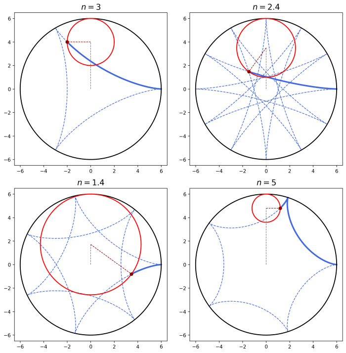 Hypocycloids with varying values of $n$. Note that $n = R/r$
Differential Length of Arc of Hypocycloid
$dL = \sqrt{\left( \dfrac{dx}{d\theta} \right)^2 + \left( \dfrac{dy}{d\theta} \right)^2} \, d\theta$
$x = a \cos \theta + r \cos b\theta$
$\dfrac{dx}{d\theta} = -a \sin \theta - br \sin b\theta = -a\left( \sin \theta + \dfrac{br}{a} \sin b\theta \right)$
$\dfrac{br}{a} = b \cdot r \cdot \dfrac{1}{a} = \dfrac{R - r}{r} \cdot r \cdot \dfrac{1}{R - r} = 1$
$\dfrac{dx}{d\theta} = -a (\sin \theta + \sin b\theta)$
$\left( \dfrac{dx}{d\theta} \right)^2 = a^2 (\sin \theta - \sin b\theta)^2 = a^2 (\sin^2 \theta + 2\sin \theta \sin b\theta + \sin^2 b\theta)$
$y = a \sin \theta - r \sin b\theta$
$\dfrac{dy}{d\theta} = a \cos \theta - br \cos b\theta = a\left( \cos \theta - \dfrac{br}{a} \cos b\theta \right)$
$\dfrac{dy}{d\theta} = a(\cos \theta - \cos b\theta)$
$\left( \dfrac{dy}{d\theta} \right)^2 = a^2 (\cos \theta - \cos b\theta)^2 = a^2 (\cos^2 \theta - 2\cos \theta \cos b\theta + \cos^2 b\theta)$
$\left( \dfrac{dx}{d\theta} \right)^2 + \left( \dfrac{dy}{d\theta} \right)^2 = a^2 (\sin^2 \theta + \cos^2 \theta) + a^2 (\sin^2 b\theta + \cos^2 b\theta) - 2a^2 (\sin \theta \sin b\theta - \cos \theta \cos b\theta)$
$\left( \dfrac{dx}{d\theta} \right)^2 + \left( \dfrac{dy}{d\theta} \right)^2 = a^2 (1) + a^2 (1) - 2a^2 (\cos b\theta \cos \theta - \sin b\theta \sin \theta)$
$\left( \dfrac{dx}{d\theta} \right)^2 + \left( \dfrac{dy}{d\theta} \right)^2 = 2a^2 - 2a^2 (\cos b\theta \cos \theta - \sin b\theta \sin \theta)$
Use the formula for the cosine of the difference of two angles
$\cos (A + B) = \cos A \cos B - \sin A \sin B$
For $A = b\theta$ and $B = \theta$:
$\cos b\theta \cos \theta + \sin b\theta \sin \theta = \cos (b\theta + \theta)$
$\cos b\theta \cos \theta + \sin b\theta \sin \theta = \cos (b + 1)\theta$
$\cos b\theta \cos \theta + \sin b\theta \sin \theta = \cos k\theta$
$\left( \dfrac{dx}{d\theta} \right)^2 + \left( \dfrac{dy}{d\theta} \right)^2 = 2a^2 - 2a^2 \cos k\theta = 2a^2 (1 - \cos k\theta)$
Use the half-angle formula
$1 - \cos \alpha = 2\sin^2 (\alpha/2)$
For $\alpha = k\theta$:
$1 - \cos k\theta = 2\sin^2 (k\theta/2)$
$\left( \dfrac{dx}{d\theta} \right)^2 + \left( \dfrac{dy}{d\theta} \right)^2 = 2a^2 \cdot 2\sin^2 \left( \dfrac{k\theta}{2} \right) = 4a^2 \sin^2 \left( \dfrac{k\theta}{2} \right)$
Hence;
$dL = \sqrt{4a^2 \sin^2 \left( \dfrac{k\theta}{2} \right)} \, d\theta$
$dL = 2a \sin \left( \dfrac{k\theta}{2} \right) \, d\theta$
Length of One Arc of Hypocycloid
$L = 2a \displaystyle \int_0^{2\pi/k} \sin \left( \dfrac{k\theta}{2} \right) \, d\theta$
$L = 2a \cdot \dfrac{2}{k} \displaystyle \int_0^{2\pi/k} \sin \left( \dfrac{k\theta}{2} \right) \, \left( \dfrac{k}{2} d\theta \right)$
$L = \displaystyle \dfrac{4a}{k} \left[ -\cos \left( \dfrac{k\theta}{2} \right) \right]_0^{2\pi/k}$
$L = \dfrac{4a}{k} \left[ -\cos \pi + \cos 0 \right] = \dfrac{4a}{k} \left[ -(-1) + 1 \right]$
$L = \dfrac{8a}{k} = 8a \cdot \dfrac{1}{k} = 8(R - r) \cdot \dfrac{r}{R}$
$L = \dfrac{8r(R - r)}{R}$
For $R = 4$ and $r = 1$:
$L = \dfrac{8(1)(4 - 1)}{4} = 6 \, \text{units}$
Manim Code for Hypocycloid of Four Cusps (Astroid)
We used AI for the Manim code while ensuring that the mathematics is fully consistent with the calculations above. In this code, we created an astroid, which is a hypocycloid with four cusps.